


An implementation of Hastie and Tibshirani’s Discriminant Adaptive Nearest Neighbor Classification in R.
In k nearest neighbors, the shape of the neighborhood is usually circular. Discriminant Adaptive Nearest Neighbor (dann) is a variation of k nearest neighbors where the shape of the neighborhood is data driven. The neighborhood is elongated along class boundaries and shrunk in the orthogonal direction. See Discriminant Adaptive Nearest Neighbor Classification by Hastie and Tibshirani.
Models:
This package implements the dann and sub-dann models described in section 4.1 of the publication and is based on Christopher Jenness’s python implementation. Calculations are done in C++ with RcppArmadillo. If R is built with OpenMP support, they are multithreaded.
Arguments:
In this example, data is simulated. The overall trend is a circle inside a square.
knitr::opts_chunk$set(echo = TRUE, fig.width = 10, fig.height = 10)
library(dann)
library(dplyr, warn.conflicts = FALSE)
library(ggplot2)
library(mlbench)

set.seed(1)

# Create training data
train <- mlbench.circle(500, 2) |>
  tibble::as_tibble()
colnames(train) <- c("X1", "X2", "Y")
train <- train |>
  mutate(Y = as.numeric(Y))

ggplot(train, aes(x = X1, y = X2, colour = as.factor(Y))) +
  geom_point() +
  labs(title = "Train Data", colour = "Y")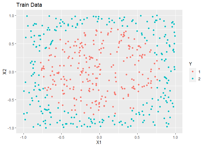
To train a model, call dann.
model <- dann(formula = Y ~ X1 + X2, data = train, k = 5, neighborhood_size = 50, epsilon = 1)To get class predictions, call predict with type equal to “class”.
# Create test data
test <- mlbench.circle(500, 2) |>
  tibble::as_tibble()
colnames(test) <- c("X1", "X2", "Y")
test <- test |>
  mutate(Y = as.numeric(Y))

yhat <- predict(object = model, new_data = test, type = "class")
yhat
#> # A tibble: 500 × 1
#>    .pred_class
#>    <fct>
#>  1 2
#>  2 2
#>  3 1
#>  4 2
#>  5 2
#>  6 2
#>  7 1
#>  8 1
#>  9 2
#> 10 1
#> # ℹ 490 more rows
To get probabilities, call predict with type equal to “prob”.
yhat <- predict(object = model, new_data = test, type = "prob")
yhat
#> # A tibble: 500 × 2
#>    .pred_1 .pred_2
#>      <dbl>   <dbl>
#>  1     0       1
#>  2     0.2     0.8
#>  3     1       0
#>  4     0       1
#>  5     0       1
#>  6     0       1
#>  7     1       0
#>  8     1       0
#>  9     0       1
#> 10     1       0
#> # ℹ 490 more rowsdann struggles when unrelated variables are intermingled with informative ones. sub_dann deals with this by projecting the data onto a lower dimensional subspace and then calling dann on that subspace. In general, it does better than dann in this situation.
Arguments:
In the example below, 2 variables are related to the outcome and 5 are not.
######################
# Circle data with unrelated variables
######################
set.seed(1)
train <- mlbench.circle(500, 2) |>
  tibble::as_tibble()
colnames(train)[1:3] <- c("X1", "X2", "Y")

# Add 5 unrelated variables
train <- train |>
  mutate(
    U1 = runif(500, -1, 1),
    U2 = runif(500, -1, 1),
    U3 = runif(500, -1, 1),
    U4 = runif(500, -1, 1),
    U5 = runif(500, -1, 1)
  )

test <- mlbench.circle(500, 2) |>
  tibble::as_tibble()
colnames(test)[1:3] <- c("X1", "X2", "Y")

# Add 5 unrelated variables
test <- test |>
  mutate(
    U1 = runif(500, -1, 1),
    U2 = runif(500, -1, 1),
    U3 = runif(500, -1, 1),
    U4 = runif(500, -1, 1),
    U5 = runif(500, -1, 1)
  )
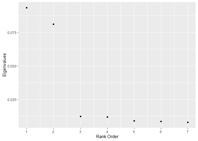
For sub_dann, the dimension of the subspace should be chosen based on the number of large eigenvalues. The graph suggests 2 (the correct answer).
knitr::opts_chunk$set(echo = TRUE, fig.width = 10, fig.height = 10)
graph_eigenvalues(
  formula = Y ~ X1 + X2 + U1 + U2 + U3 + U4 + U5,
  data = train,
  neighborhood_size = 50,
  weighted = FALSE,
  sphere = "mcd"
)
dann_model <- dann(
  formula = Y ~ X1 + X2 + U1 + U2 + U3 + U4 + U5,
  data = train,
  k = 3,
  neighborhood_size = 50,
  epsilon = 1
)
# numDim based on large eigenvalues
# weighted, sphere, and neighborhood_size kept consistent between sub_dann and graph_eigenvalues
sub_dann_model <- sub_dann(
  formula = Y ~ X1 + X2 + U1 + U2 + U3 + U4 + U5,
  data = train,
  k = 3,
  neighborhood_size = 50,
  epsilon = 1,
  weighted = FALSE,
  sphere = "mcd",
  numDim = 2
)
As expected, the dann model fit on all seven variables has the lower AUC.
library(yardstick)
dann_yhat <- predict(object = dann_model, new_data = test, type = "prob")
dann_yhat <- test |>
  select(Y) |>
  bind_cols(dann_yhat)
roc_auc(data = dann_yhat, truth = Y, event_level = "first", .pred_1)
#> # A tibble: 1 × 3
#>   .metric .estimator .estimate
#>   <chr>   <chr>          <dbl>
#> 1 roc_auc binary         0.864
sub_dann, fit on the two dimensional subspace, does better.
sub_dann_yhat <- predict(object = sub_dann_model, new_data = test, type = "prob")
sub_dann_yhat <- test |>
  select(Y) |>
  bind_cols(sub_dann_yhat)
roc_auc(data = sub_dann_yhat, truth = Y, event_level = "first", .pred_1)
#> # A tibble: 1 × 3
#>   .metric .estimator .estimate
#>   <chr>   <chr>          <dbl>
#> 1 roc_auc binary         0.933