---
title: "Similarity Matrices"
output:
rmarkdown::html_vignette:
toc: true
description: >
Visualize the affinity matrices produced by SNF and how they associate with other data attributes.
vignette: >
%\VignetteIndexEntry{Similarity Matrices}
%\VignetteEngine{knitr::rmarkdown}
%\VignetteEncoding{UTF-8}
---
```{r setup, include=FALSE}
knitr::opts_chunk$set(echo = TRUE)
```
```{r echo = FALSE}
options(crayon.enabled = FALSE, cli.num_colors = 0)
```
Download a copy of the vignette to follow along here: [similarity_matrix_heatmaps.Rmd](https://raw.githubusercontent.com/BRANCHlab/metasnf/refs/heads/main/vignettes/similarity_matrix_heatmap.Rmd)
This vignette walks through usage of `similarity_matrix_heatmap` to visualize the final similarity matrix produced by a run of SNF and how that matrix associates with other patient attributes.
## Data set-up
```{r}
library(metasnf)
# Generate data_list
my_dl <- data_list(
list(
data = expression_df,
name = "expression_data",
domain = "gene_expression",
type = "continuous"
),
list(
data = methylation_df,
name = "methylation_data",
domain = "gene_methylation",
type = "continuous"
),
list(
data = gender_df,
name = "gender",
domain = "demographics",
type = "categorical"
),
list(
data = diagnosis_df,
name = "diagnosis",
domain = "clinical",
type = "categorical"
),
list(
data = age_df,
name = "age",
domain = "demographics",
type = "discrete"
),
uid = "patient_id"
)
set.seed(42)
my_sc <- snf_config(
my_dl,
n_solutions = 1,
max_k = 40
)
sol_df <- batch_snf(
my_dl,
my_sc,
return_sim_mats = TRUE
)
similarity_matrices <- sim_mats_list(sol_df)
# The first (and only) similarity matrix:
similarity_matrix <- similarity_matrices[[1]]
# The first (and only) cluster solution:
cluster_solution <- t(sol_df)
```
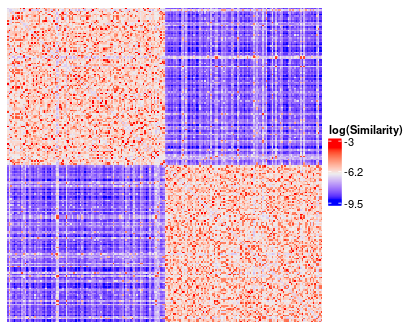
## Visualize similarity matrices sorted by cluster label
`similarity_matrix_heatmap` is a wrapper for `ComplexHeatmap::Heatmap`, but with some convenient default transformations and parameters for viewing a similarity matrix.
```{r eval = FALSE}
similarity_matrix_hm <- similarity_matrix_heatmap(
similarity_matrix = similarity_matrix,
cluster_solution = cluster_solution,
heatmap_height = grid::unit(10, "cm"),
heatmap_width = grid::unit(10, "cm")
)
```
```{r eval = FALSE, echo = FALSE}
save_heatmap(
heatmap = similarity_matrix_hm,
path = "vignettes/similarity_matrix_heatmap.png",
width = 410,
height = 330,
res = 80
)
```
<center>
</center>
The default transformations include plotting log(Similarity) rather than the default similarity matrix as well as rescaling the diagonal of the matrix to the average value of the off-diagonals.
Additionally, the similarity matrix gets reordered according to the provided cluster solution.
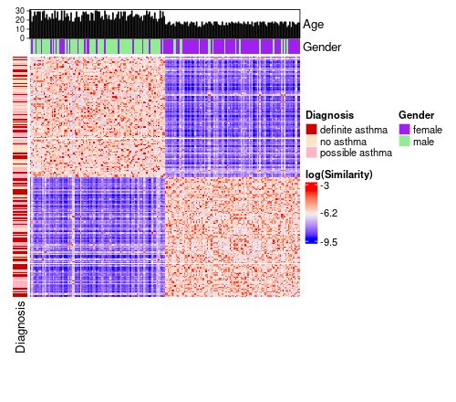
## Annotations
One piece of functionality provided by `ComplexHeatmap::Heatmap()` is the ability to supply visual annotations along the rows and columns of a heatmap.
You can always build annotations using the standard approaches outline in the [ComplexHeatmap Complete Reference](https://jokergoo.github.io/ComplexHeatmap-reference/book/index.html).
In addition to that, this package offers some convenient functionality to specify regular heatmap annotations and barplot annotations directly through a provided data frame or data_list (or both).
In the example below, we make use of data supplied through a data list.
```{r eval = FALSE}
annotated_sm_hm <- similarity_matrix_heatmap(
similarity_matrix = similarity_matrix,
cluster_solution = cluster_solution,
scale_diag = "mean",
log_graph = TRUE,
data = my_dl,
left_hm = list(
"Diagnosis" = "diagnosis"
),
top_hm = list(
"Gender" = "gender"
),
top_bar = list(
"Age" = "age"
),
annotation_colours = list(
Diagnosis = c(
"definite asthma" = "red3",
"possible asthma" = "pink1",
"no asthma" = "bisque1"
),
Gender = c(
"female" = "purple",
"male" = "lightgreen"
)
),
heatmap_height = grid::unit(10, "cm"),
heatmap_width = grid::unit(10, "cm")
)
```
```{r eval = FALSE, echo = FALSE}
save_heatmap(
heatmap = annotated_sm_hm,
path = "vignettes/annotated_sm_heatmap.png",
width = 500,
height = 440,
res = 80
)
```
<center>
</center>
The colours `red3`, `pink1`, etc. are built-in R colours that you can browse by calling `colours()`.
For reference, the code below shows how you would achieve these annotations using standard `ComplexHeatmap` syntax.
```{r eval = FALSE}
merged_df <- as.data.frame(my_dl)
order <- sort(cluster_solution[, 2], index.return = TRUE)$"ix"
merged_df <- merged_df[order, ]
top_annotations <- ComplexHeatmap::HeatmapAnnotation(
Age = ComplexHeatmap::anno_barplot(merged_df$"age"),
Gender = merged_df$"gender",
col = list(
Gender = c(
"female" = "purple",
"male" = "lightgreen"
)
),
show_legend = TRUE
)
left_annotations <- ComplexHeatmap::rowAnnotation(
Diagnosis = merged_df$"diagnosis",
col = list(
Diagnosis = c(
"definite asthma" = "red3",
"possible asthma" = "pink1",
"no asthma" = "bisque1"
)
),
show_legend = TRUE
)
similarity_matrix_heatmap(
similarity_matrix = similarity_matrix,
cluster_solution = cluster_solution,
scale_diag = "mean",
log_graph = TRUE,
data = merged_df,
top_annotation = top_annotations,
left_annotation = left_annotations
)
```
Take a look at the [ComplexHeatmap Complete Reference](https://jokergoo.github.io/ComplexHeatmap-reference/book/index.html) to learn more about what is possible with this package.
## More on sorting
Be aware that the ordering of both your data and your similarity matrix will be influenced if you supply values for the `cluster_solution` or `order` parameters.
If you don't think your data is lining up properly, consider manually making sure your `similarity_matrix` rows and columns are sorted to your preference (e.g., based on cluster) and that the order of your data matches.
This will be easier to do with a `data frame` than with a `data_list`, as the `data_list` forces patients to be sorted by their unique IDs upon generation.