2018-04-18
To understand the concept of p value is very important. To teach the the distribution of common statistic( \(\chi^2\) for chisq.test() , t for Student’s t-test , F for F-test) and concept of the p-value, plot.htest() function can be used.
https://cardiomoon.github.io/webr/index.html
You can install this package form the github. Currently, package
webr is under construction and consists of only one
function - plot.htest().
#install.packages("devtools")
devtools::install_github("cardiomoon/webr")The plot.htest() function is a S3 method for class “htest”. Currently, this function covers Welch Two Sample t-test, Pearson’s Chi-squared test, Two Sample t-test, One Sample t-test, Paired t-test and F test to compare two variances.
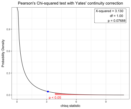
You can show the distribution of chi-squre statistic and p-value.
 require(moonBook)
 require(webr)

 # chi-squared test
 x=chisq.test(table(acs$sex,acs$DM))
 x
    Pearson's Chi-squared test with Yates' continuity correction

data:  table(acs$sex, acs$DM)
X-squared = 3.1296, df = 1, p-value = 0.07688 plot(x)
You can show the distribution of t-statistic and p-value in one sample t-test.
t.test(acs$age,mu=63)
    One Sample t-test

data:  acs$age
t = 0.77978, df = 856, p-value = 0.4357
alternative hypothesis: true mean is not equal to 63
95 percent confidence interval:
 62.52736 64.09574
sample estimates:
mean of x
63.31155 plot(t.test(acs$age,mu=63))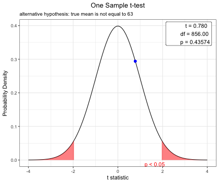
Before performing a t-test, you have to compare two variances.
x=var.test(age~DM,data=acs)
x
    F test to compare two variances

data:  age by DM
F = 1.2383, num df = 552, denom df = 303, p-value = 0.0376
alternative hypothesis: true ratio of variances is not equal to 1
95 percent confidence interval:
 1.012416 1.505776
sample estimates:
ratio of variances
1.238288 plot(x)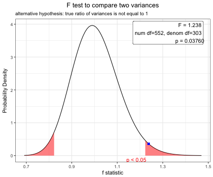
Based on the result of var.test(), you can perform t.test with default option(var.equal=FALSE).
x=t.test(age~DM,data=acs)
x
    Welch Two Sample t-test

data:  age by DM
t = 0.58982, df = 682.36, p-value = 0.5555
alternative hypothesis: true difference in means is not equal to 0
95 percent confidence interval:
 -1.112568  2.068014
sample estimates:
 mean in group No mean in group Yes
63.48101 63.00329 plot(x)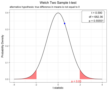
To compare means of body-mass index between male and female patients, perform F test first.
var.test(BMI~sex,data=acs)
    F test to compare two variances

data:  BMI by sex
F = 1.2078, num df = 254, denom df = 508, p-value = 0.07756
alternative hypothesis: true ratio of variances is not equal to 1
95 percent confidence interval:
 0.9794315 1.5008098
sample estimates:
ratio of variances
1.207759 plot(var.test(BMI~sex,data=acs))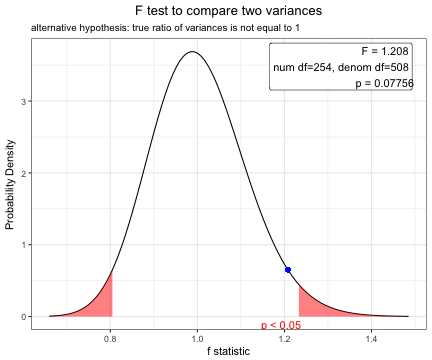 Based on the result of F test, you can perform t-test using pooled
variance.
x=t.test(BMI~sex,data=acs,var.equal=TRUE)
x
    Two Sample t-test

data:  BMI by sex
t = -0.50823, df = 762, p-value = 0.6114
alternative hypothesis: true difference in means is not equal to 0
95 percent confidence interval:
 -0.6348532  0.3737344
sample estimates:
mean in group Female   mean in group Male
24.19492 24.32548 plot(x)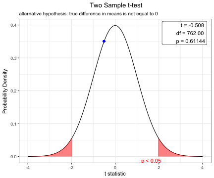
You can show the distribution of t-statistic and p-value in paired t-test.
x=t.test(iris$Sepal.Width,iris$Petal.Width,paired=TRUE)
plot(x)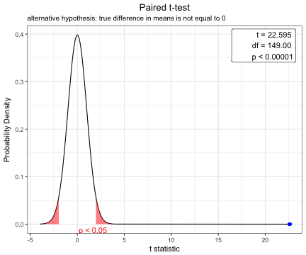
You can change the options of t.test.
x=t.test(BMI~sex, data=acs,conf.level=0.99,alternative="greater",var.equal=TRUE)
plot(x)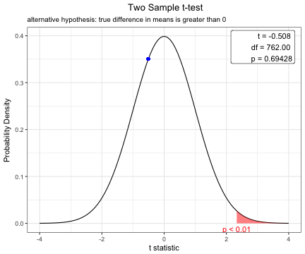
http://rpubs.com/cardiomoon/398623